Predicting diabetes outcomes with machine learning

Understanding the dataset

This dataset is originally from the National Institute of Diabetes and Digestive and Kidney Diseases. The objective is to predict based on diagnostic measurements whether a patient has diabetes.

Several constraints were placed on the selection of these instances from a larger database. In particular, all patients here are females at least 21 years old of Pima Indian heritage.

Pregnancies: Number of times pregnant
Glucose: Plasma glucose concentration a 2 hours in an oral glucose tolerance test
BloodPressure: Diastolic blood pressure (mm Hg)
SkinThickness: Triceps skin fold thickness (mm)
Insulin: 2-Hour serum insulin (mu U/ml)
BMI: Body mass index (weight in kg/(height in m)^2)
DiabetesPedigreeFunction: Diabetes pedigree function
Age: Age (years)
Outcome: Class variable (0 or 1)

Let’s load in the data and libraries:

library(tidyverse)
library(ggplot2)
library(ggcorrplot)
library(tidymodels)
library(tune)

diabetes_data <- read.csv(".../diabetes.csv")

str(diabetes_data)

Looking at the structure tells us that outcome (which should be a factor) is stored as an integers. We’ll change that first.

diabetes_data$Outcome <- as.factor(diabetes_data$Outcome)

Including Plots

It’s good practice to do some exploratory data analysis when first beginning with a dataset. Thankfully the PIMA dataset is pretty clean and doesn’t contain any missing values. Still, there are some things that I’d like to know to get a better sense of what I’m working with.

ggplot(aes(x = Age), data=diabetes_data) +
        geom_histogram(binwidth=1, fill = "#A11F7F", alpha = .6) +
        scale_x_continuous(limits=c(20,90), breaks=seq(20,90,5), expand = c(0, 0)) +
        scale_y_continuous(expand = c(0, 0)) +
        labs(x = "Age",
             y = "Number of people\n",
             title = "Distribution by age") +

  theme_classic() +
  theme(title = element_text(size = 28)) +
  theme(axis.ticks = element_blank()) +
  theme(axis.text = element_text(size = 23)) +
  theme(axis.title = element_text(size = 26)) +
  theme(panel.grid.minor.x = element_blank()) +
  theme(axis.line.y = element_blank()) +
  theme(legend.text = element_text(size = 16)) +
  theme(legend.title = element_text(size = 20)) +
  theme(axis.ticks = element_blank()) +
  theme(legend.position = c(.9, .7)) +
  theme(legend.text = element_text(size = 20)) +
  theme(legend.text = element_text(margin = margin(t = 10)))

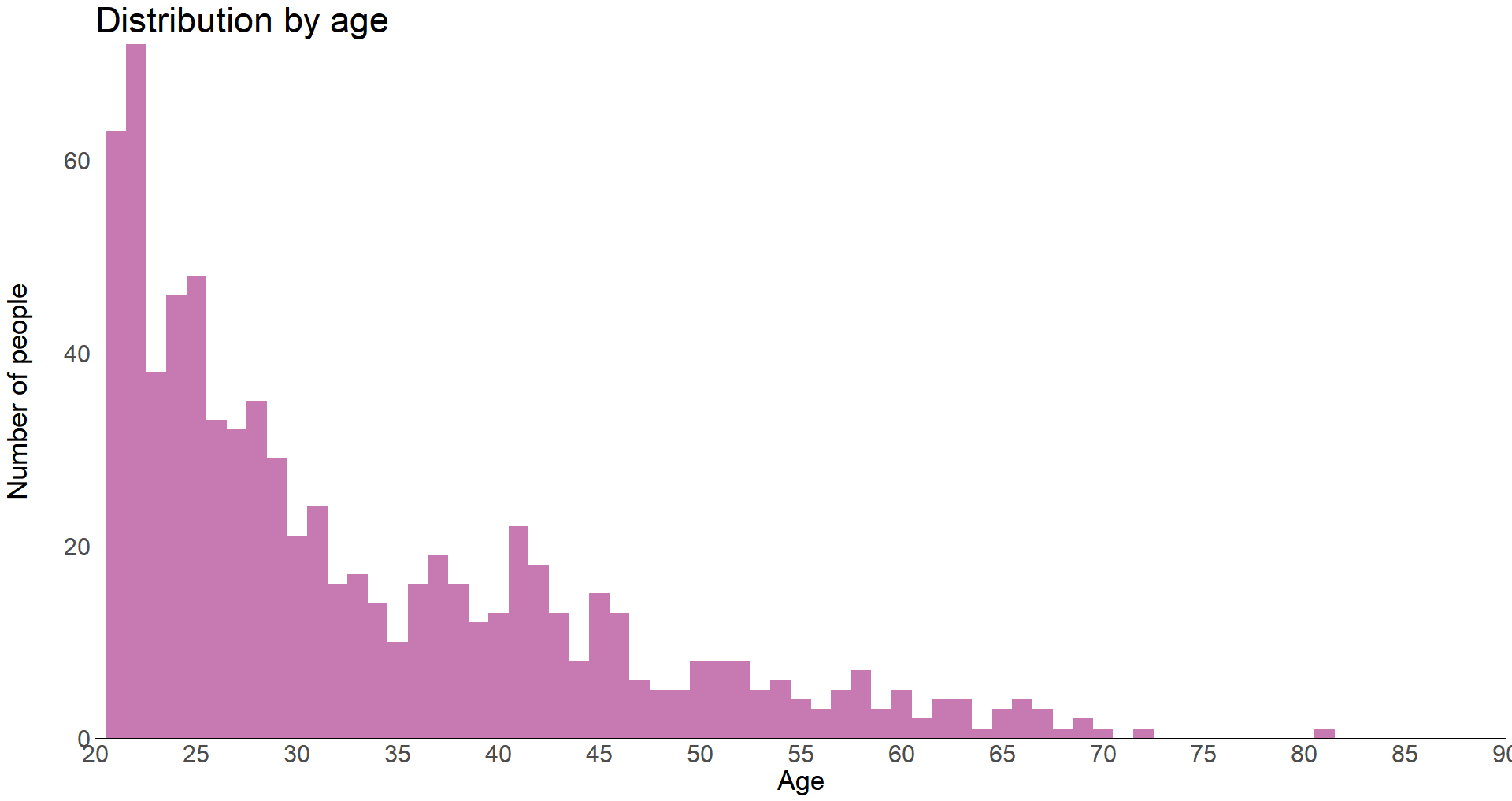
We can see that most of the test subjects are young, between 21-30 years old. Let’s group up the ages to make it easier to derive conclusions from the data.

# Create Age Category column
diabetes_data$Age_Cat <- ifelse(diabetes_data$Age < 21, "<21", 
                   ifelse((diabetes_data$Age>=21) & (diabetes_data$Age<=25), "21-25", 
                   ifelse((diabetes_data$Age>25) & (diabetes_data$Age<=30), "25-30",
                   ifelse((diabetes_data$Age>30) & (diabetes_data$Age<=35), "30-35",
                   ifelse((diabetes_data$Age>35) & (diabetes_data$Age<=40), "35-40",
                   ifelse((diabetes_data$Age>40) & (diabetes_data$Age<=50), "40-50",
                   ifelse((diabetes_data$Age>50) & (diabetes_data$Age<=60), "50-60",">60")))))))

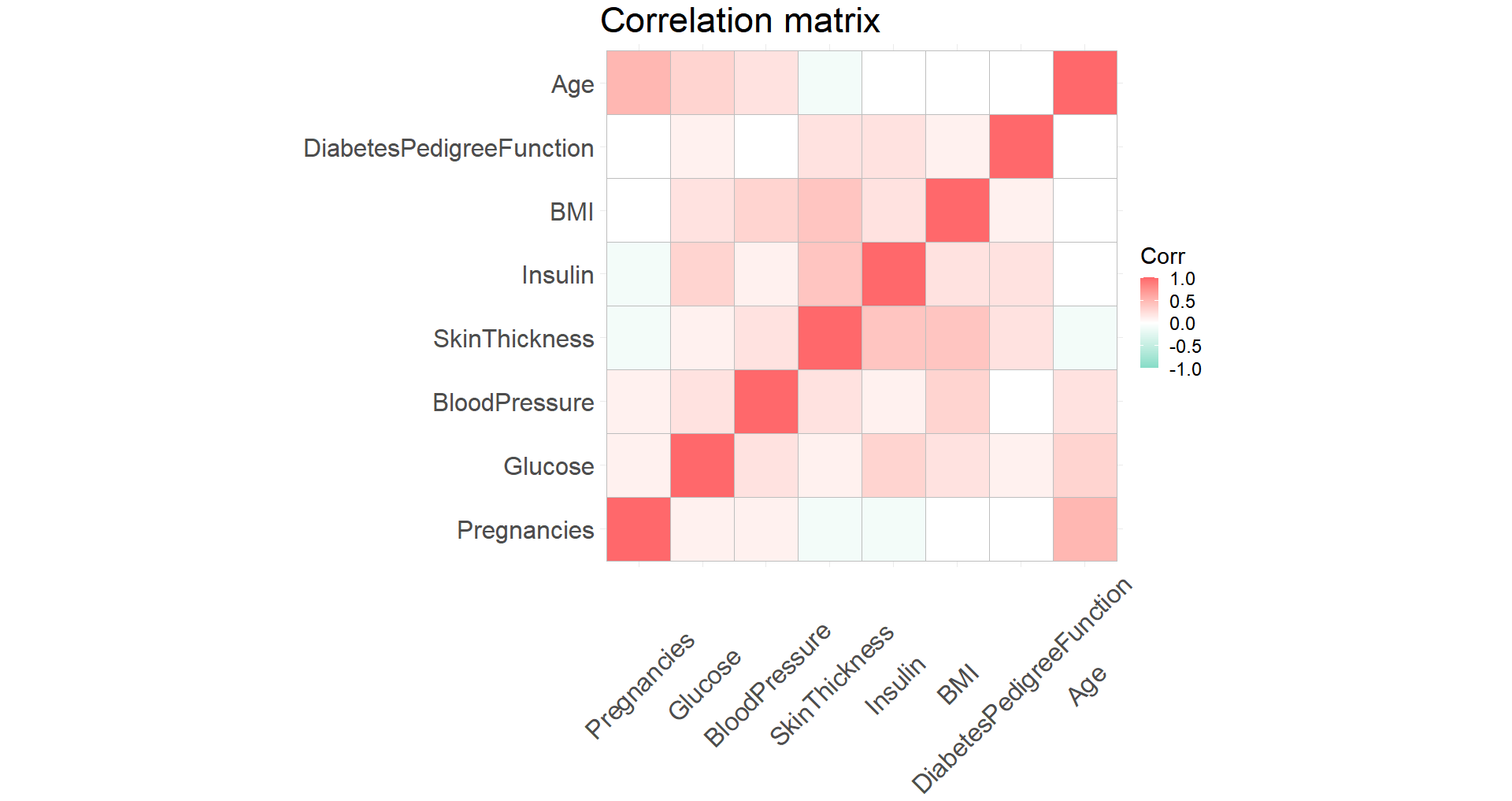
A correlation plot shows that the variables are not too strongly correlated with each other so we’ll keep them all for now.

# Compute correlation matrix
db_cor <- round(cor(diabetes_data[1:8]),1)

ggcorrplot(db_cor, colors = c("#84dcc6", "white", "#ff686b")) 

Predicting diabetes outcomes with maching learning

We’ll use a logistic regression to see if we can successfully predict who is likely to have diabetes based on our data. To start, let’s split the data into training and testing samples and we’ll strata based on Outcome.

diabetes_split <- diabetes_data %>%
  initial_split(strata = Outcome)

diabetes_train <- training(diabetes_split) 
diabetes_test <- testing(diabetes_split) 

Next let’s set up the logistic regression as glm_spec and fit it to the data. We’re estimating Outcome as a function of the rest of the explanatory variables.

glm_spec <- logistic_reg() %>%
  set_engine(engine = 'glm')

logistic_fit <- glm_spec %>%
  fit(Outcome ~ ., 
      data = diabetes_train)

Now let’s try a random forest model for classification. Again, fit the random forest model on our equation estimating Outcome as a function of the rest of the variables.

rf_spec <- rand_forest(mode = "classification") %>%
  set_engine("ranger") 

rf_fit <- rf_spec %>%
  fit(Outcome ~ ., 
      data = diabetes_train)

Great! We can use different metrics to gauge how the two models performed. For this, we create a new variable called custom_metrics which uses metric_set from the yardstick package.

To discern the models, we can take results_train and group by model type then simply apply our metrics to the two models.

custom_metrics <- metric_set(accuracy, sens, spec, precision, recall, f_meas, kap, mcc)

results_train %>%
  group_by(model) %>%
  custom_metrics(truth = true_outcome,
                 estimate = .pred_class)

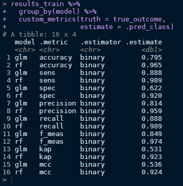
It looks like the random forest model outperformed the logistic model across all fronts! Not that that’s unexpected since random forests can learn better than logistic models.

Bootstrapping

The models we already have perform well, but creating bootstraps with resampling will allow us to better compare them. What we’re doing here is creating splits and randomly selecting a subset of the data, making sure to resample with replacement. We get 25 total bootstraps with a sample size of 576.

diabetes_boot <- bootstraps(diabetes_train)

We’ll create a workflow with out formula (Outcome regressed on all our explanatory variables) and use that as an input in both a logistic and random forest model. From there we’ll fit the resamples generated by bootstrapping and compare the performance between the two models with collect_metrics.

diabetes_wf <- workflow() %>%
  add_formula(Outcome ~ .) 

glm_results <- diabetes_wf %>%
  add_model(glm_spec) %>%
  fit_resamples(
    resamples = diabetes_boot,
    control = control_resamples(save_pred = T)
  )

rf_results <- diabetes_wf %>%
  add_model(rf_spec) %>%
  fit_resamples(
    resamples = diabetes_boot,
    control = control_resamples(save_pred = T)
  )
  
collect_metrics(glm_results)
collect_metrics(rf_results)

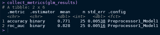
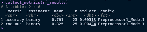
Looks like logistic model performs better in this case!

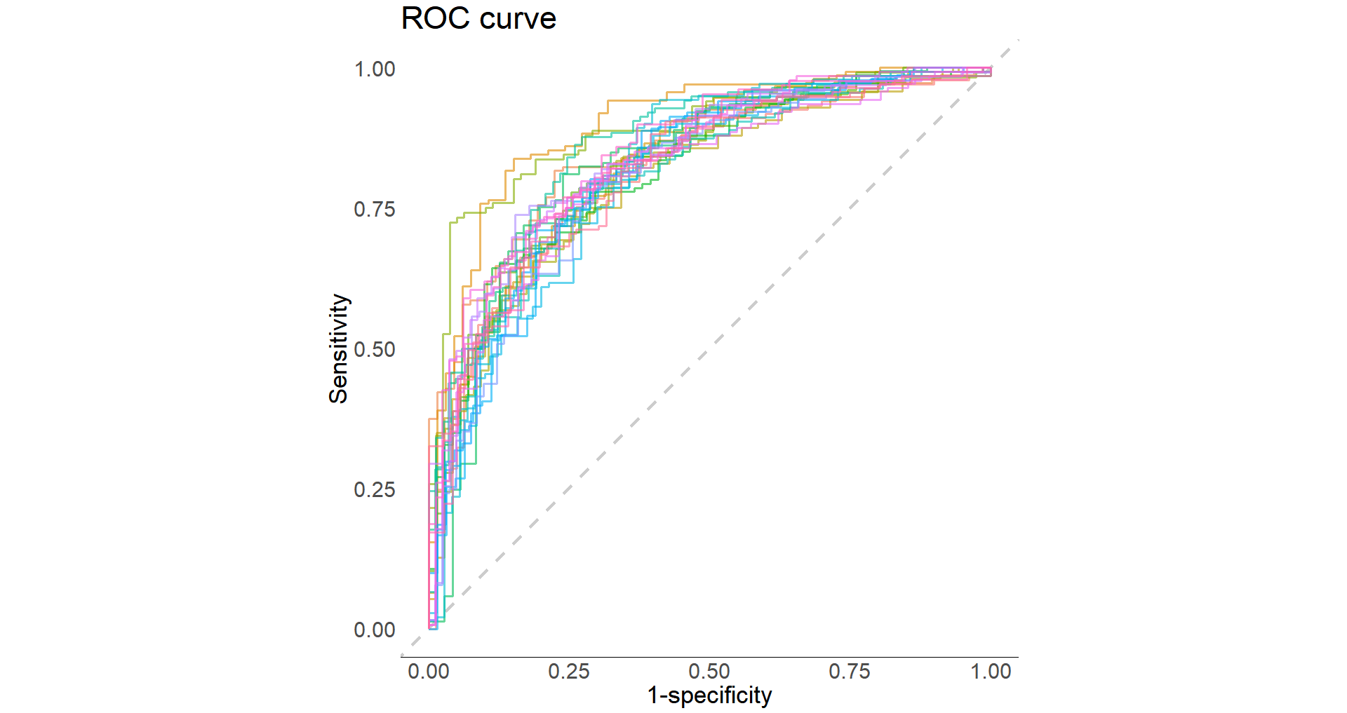
Plot ROC curve:

glm_results %>%
  collect_predictions() %>%
  group_by(id) %>%
  roc_curve(Outcome, .pred_0) %>%
  autoplot()

Now let’s fit the best model to the testing dataset:

diabetes_final <- diabetes_wf %>%
                    add_model(glm_spec) %>%
                    last_fit(diabetes_split)

diabetes_final

collect_metrics(diabetes_final)

collect_predictions(diabetes_final) %>%
  conf_mat(Outcome, .pred_class)

Get the fitted workflow:

diabetes_final$.workflow[[1]] %>%
  tidy(exponentiate = T) %>%
  filter(p.value < .1)

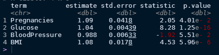
We can extract our model estimates and tidy up the results by exponentiating them makes it a little to make it easier to read as it gives the odds ratio. Keeping those variables with a p-value < .1 results in four significant features (Pregnancies, Glucose, BloodPressure, and BMI). So using our best logistic model we can now make some interpretations.

First off, all our estimates are positives which means that all four of these variables are will increase the chance of being diabetic. So what’re the results telling us here? Every pregnancy that a woman has had results in about a 9% increase in the odds of a woman being diabetic. A one unit increase in blood glucose levels results in a ~3% increase in the odds of being diabetic. For every mm Hg (unit of blood pressure) increase, the chance of we expect to see a 0.99% increase in the odds of being diabetic. And lastly, for every unit increase in BMI, we’d expect a 8% increase in the odds of being diabetic.